01Methods
- Closed form with continuous dividend yield and analytic delta, gamma, vega, theta, rho.
- CRR lattice, vectorised over each layer, with an early-exercise check for American options.
- Monte Carlo under GBM: plain; antithetic pairs; and ST as a control variate, whose discounted mean is known exactly (S·e−qT).
- Implied vol: Newton steps on vega from σ = 20%, falling back to bisection when vega vanishes or a step leaves (0.01%, 500%).
02Convergence and variance reduction
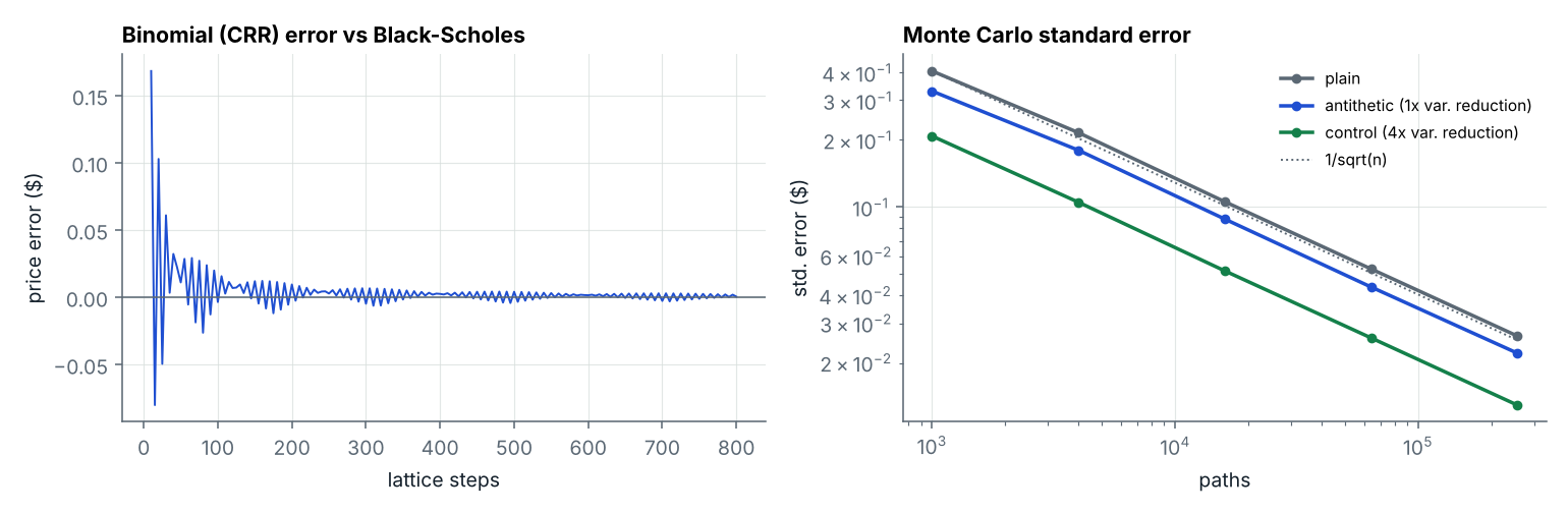
At 256,000 paths the standard error is $0.0264 plain, $0.0221 antithetic and $0.0129 with the control variate. Antithetic helps less here because the payoff is far from linear in the shock.
03Greeks
04Implied volatility edge case
Over 2,034 strike, volatility and expiry combinations the solver recovers σ to within 7e-07. It skips 198 cases on purpose: deep in- or out-of-the-money options at low volatility are worth their intrinsic value to machine precision, so no volatility can be recovered from the price. The first test run failed on exactly these cases, which is how I found them.
def implied_vol(price, S, K, T, r, q=0.0, kind="call"):
    # reject prices outside no-arbitrage bounds, then Newton on vega
    sig = 0.2
    for _ in range(max_iter):
        diff = bs_price(S, K, T, r, sig, q, kind) - price
        if abs(diff) < tol: return sig
        v = bs_greeks(S, K, T, r, sig, q, kind)["vega"]
        if v < 1e-8: break          # flat region: fall back to bisection
        sig -= diff / v
Swapping SciPy's distribution objects for scipy.special.ndtr cut the solve time from 2.7 ms to 81 µs.
05What I'd do next
- Heston pricing via characteristic functions and the Carr-Madan FFT.
- Fit an SVI smile to real option quotes and check for static arbitrage.
- Delta-hedging P&L under misspecified volatility.